Speech morphing with STRAIGHT

In this tutorial, I will show you how to morph two speech samples into one another and create in between versions of the two recordings using STRAIGHT toolbox for MATLAB.

About STRAIGHT

Several different versions of STRAIGHT software exist (e.g., legacy-STRAIGHT), which contain earlier or later implementations of the speech morphing algorithms. In this tutorial, I'm using one of the latest versions called TANDEM-STRAIGHT that introduced two significant improvements over its predecessors: (1) TANDEM and (2) a new spectral envelope recovery method (Kawahara, Takahashi, Morise, & Banno, 2009). As the authors explained, “TANDEM is a simple method for yielding a temporally static power spectral representation of periodic signals by averaging two power spectra calculated at temporal positions 0.5/F0 apart. The spectral envelope recovery method is based on a new formulation of sampling theory called “consistent sampling” (Unser, 2000), which only requires recovery at resampled points of D/A results” (Kawahara et al., 2009, p. 112). These revisions enable temporally variable multi-aspect morphing without introducing objective and perceptual breakdown.

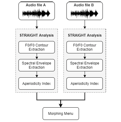
Main analyses can be performed either from the TandemSTRAIGHTHandler program or from the MorphingMenu program. The former module is used to decompose each input audio file into three high-level acoustic features – F0 contour, aperiodicity index and spectral envelope, which are then used to detect voiced and unvoiced breakpoints and the duration of each voiced or unvoiced part of speech. This decomposition is necessary before launching the latter module, which uses this derived high-level structure to warp all the features in time using the information of breakpoints and pre-processes to re-scale the values along the selected dimensions. STRAIGHT allows morphs along several dimensions: Aperiodicity, Spectrum, Frequency, Time (duration), and F0 (pitch).

Preparations

All versions of this software are MATLAB packages, so you need to have MATLAB or Octave installed to be able to use it. To begin, download the STRAIGHT package and unzip the folder in your chosen location. Next, add the folder containing STRAIGHT to your MATLAB path to ensure the software can access its functions. Prepare pairs of stimuli for morphing by using cleaned and normalised recordings that have no silences at the beginning or end. Then, create a dedicated folder to store your initial stimuli (all in WAV format), which you will use for morphing. This same folder will also be used to save all output files generated during the STRAIGHT analysis. Be sure to add this folder to your MATLAB path as well, so that MATLAB can locate your stimuli and process them correctly.

Part I: STRAIGHT analysis

The first part of this tutorial explains how to do the analysis of sound files to extract the F0 contour, aperiodicity index and spectral envelope through the TandemSTRAIGHTHandler program. At the end of this analysis pipeline, you should have extracted the high-level control structure from each speech sample and saved the results as .mat files. Then, you can load those .mat files along with the wav files to the MorphingMenu program to create morphed continua of the stimuli.

Note: STRAIGHT analysis has to be repeated for each audio stimulus.

First, STRAIGHT automatically extracts F0 values with fixed-point analysis (Kawahara, Katayose, de Cheveigne, & Patterson, 1999). F0 adaptive window is used to minimize the interference with spectral envelope. If we analyze exactly the same speech sound, but at different F0, STRAIGHT will produce the same spectral envelope. That means that F0 and spectral envelope are statistically independent, which is essential for modelling we will do later where we assume that independence. STRAIGHT is doing a good job at separating these two parameters.

STRAIGHT is a source-filter model, but the filter it uses is not a vocal tract filter but a simple spectral envelope filter (more general than vocal tract). Using the extracted F0 values STRAIGHT carries out F0-adaptive spectral analysis combined with a surface reconstruction method in the time-frequency region to remove signal periodicity.

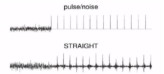
It also extracts aperiodicity measurements on the frequency domain. Instead of having to switch between aperiodic energy and purely periodic energy (the pulse or noise vocoder, see figure below), STRAIGHT mixes the two together, and the ratio at which they combine serves as one of the parameters of the vocoder (i.e., the ratio between periodic and aperiodic energy at each frequency). That ratio is different at different frequency bands, and it represents the relative energy distribution of aperiodic signal components (Kawahara, Estill, & Fujimura, 2001). Additionally, instead of using actual pulses, STRAIGHT manipulates the phases of the sinewaves that make up these pulses (it blurs them a little but maintains the magnitude and spectrum as pulse trains). This helps with generating less “buzzing” in the synthesized speech.

Because of these parameters, STRAIGHT is quite good at generating smooth transitions between voiced and unvoiced sounds. We observe only partial signal loss after speech reconstruction (relatively natural-sounding speech, but with still audible “buzziness”). Some better models have the potential to reconstruct the speech signal with perceptually better quality (e.g., sinusoidal models) but are more difficult to implement due to multiple varying parameters.

1.1. Initialising STRAIGHT analysis module

To invoke the menu interface for the analysis, type the following in the MATLAB Command Window: TandemSTRAIGHThandler.

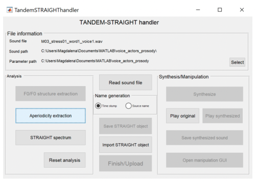
The Select sound file tab will open in which you need to select the first audio file you want to analyze. Navigate to the folder where you store your prepared pair of stimuli for morphing and select the first one. Once the selection is made, the following interface should open (see Figure 3). Only relevant buttons are accessible depending on the stage of processing (the rest is grayed out).

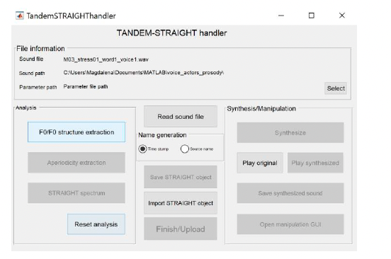
Note: The File information section contains information about the audio file you are currently analyzing (Sound file), its location (Sound path) and the location of the folder to which STRAIGHT will save all the output files from the analysis (Parameter path). The Analysis section consists of three stages of analysis – F0/F0 structure extraction, Aperiodicity extraction and STRAIGHT spectrum. The Reset analysis button below allows you to reject all the analyses you conducted so far and start from the beginning. You can check if you loaded the correct file by pressing the Play original button in the Synthesis/Manipulation section. If you loaded a wrong audio file by mistake, you can reload it by clicking the Read sound file button in the middle, which brings back the Select sound file tab.

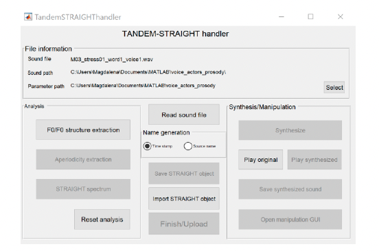
Click the Select button on the left (next to Parameter path) to tell MATLAB where you want to save all the resulting files. An updated window should now have the name of the folder you selected (see Figure 4).

Note: This window (TandemSTRAIGHThandler) remains open in the background throughout the next steps of the analysis – please do not close this!

1.2. F0/F0 structure extraction

To start the F0/F0 structure extraction, press the appropriate button in the Analysis section. Pressing this button opens a new f0ExtractorGUI tab in MATLAB (see Figure 5).

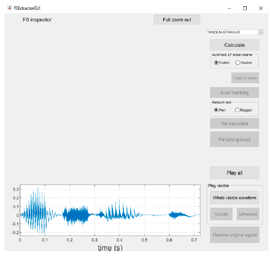
Note: At this point, the only available option is the Play all button. You can listen to the audio file you just loaded.

As a first step, please press the Calculate button. This generates an initial pitch track and highlights the voiced and unvoiced regions of the waveform (see Figure 6). This might take a few seconds, so please be patient and don’t click any other buttons while MATLAB is processing your request.

Note: The middle panel shows the extracted F0 trajectory (represented with a thick cyan-coloured line). Other F0 candidates that represent local periodicity are plotted using coloured dots. The colour of the dots represents the order of the periodicity level of each candidate. The periodicity levels and the colour order are shown in the top panel.

The resulting pitch track is usually quite good, but it might require some tweaking to guarantee smoother morphing effects. What STRAIGHT has done so far is that it recognized most of the voiced sections. The voiced parts of speech (vowels and voiced consonants) are highlighted with the green frames in the bottom panel, which correspond to the clear extracted pitch contours in the middle panel (horizontal lines connecting orange points arranged closely one next to another). The unvoiced parts of speech (unvoiced consonants or pauses) are outside the green boxes in the bottom panel (flat green lines) and are represented by multiple vertical lines in the middle panel – this is because there is no clear pitch signature in unvoiced parts of speech.

Next, we click the Clean LF noise button to clean the low-frequency noise. It does not make a lot of difference in the overall result, but it removes some general low-frequency background noise that we don’t want to model. After this is done, all other buttons will turn grey, so you need to press the Calculate button again to re-calculate and enable further analyses.

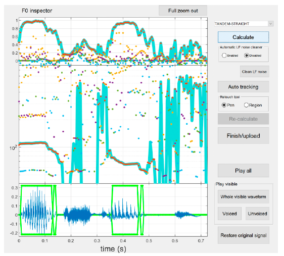
The next step is to apply Auto tracking to clean up the pitch track (see Figure 7). This works pretty well, but there might be some errors in selecting frames with voiced (all voiced content should be included within the green frame) vs unvoiced (these are the flat green parts) contents, which should be corrected manually.

At this point, you might want to listen to these to check if all voiced regions have been appropriately selected and how well your analysis worked so far. You can do it by pressing one of the buttons on the bottom left, either Play all or one of the buttons below the Play visible header – Play visible (plays the whole waveform), Voiced (placed only the parts selected as voiced), or Unvoiced (plays only the parts selected as unvoiced).

To adjust the selection of voiced vs unvoiced regions (bottom panel), you can click the edge of a voiced region (green frame) and drag it around. To delete these regions, I find it easiest to drag one of the voiced regions from the vowel over the erroneous regions and then drag it back to where it should be. You can also click the right side of a voiced interval and drag it all the way to the left side of it, which will remove all of it. See below for more details on how to interact with the F0 extraction interface.

F0 extraction interface controls:

• Zoom in/out
  • Click on the time axis to zoom in
  • Hold shift and click to zoom out
  • Click and drah to move the visible part of the waveform
• Extend/reduce a voiced portion
  • Click and drag a boundary to extend/reduce a voiced portion
  • Moving a boundary over another voiced portion will overwrite it, which can help with deleting lots of small voiced portions
• Click and drag a point to mark a frame as either unvoiced or voiced
  • Drag to the centre to mark as unvoiced
  • Drag to top or bottom to mark as voiced

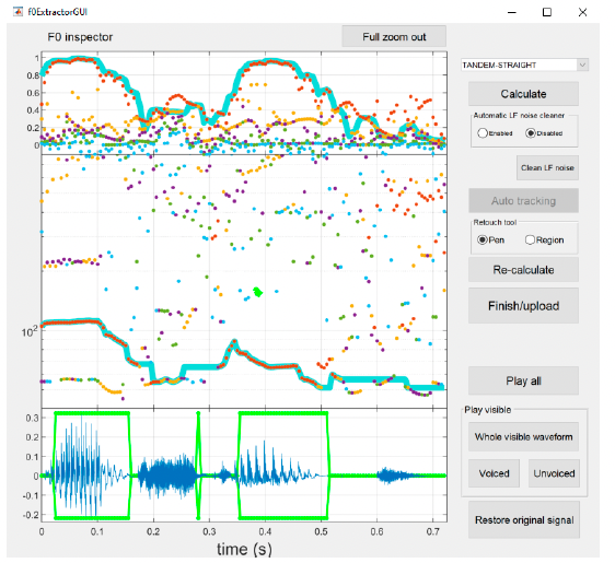
To adjust the pitch track (middle panel), you can use the Retouch tool (pen or region) to point to problematic parts of the selection manually. It should be especially helpful for creaky voices to draw the lines where f0 is not detectible (this might be an issue for whispered voices as well). Once you make some manual changes, the Re-calculate option becomes available, and you need to click it to re-calculate the pitch track to incorporate all the changes you made using retouching markers (see Figure 8).

Once you are satisfied with your analysis, press the Finish/Upload button to upload the extracted F0 contour into STRAIGHT.

Note: If you are still unhappy with the effects of your analysis, you can apply some additional corrections and then re-calculate again. However, please don't overdo it because by applying too many changes, you might introduce some unwanted distortions. If things go awry, you can always go back to the original file and start from scratch by pressing the Restore original sample button in the bottom left corner of the f0ExtractorGUI.

After you're done, you will come back to the TandemSTRAIGHThandler tab you had open all this time in the background, but now a few new options became available (see Figure 9).

1.3. Aperiodicity index

The next step of analysis is aperiodicity extraction. Aperiodic portions of the signal are extracted and analyzed by estimating a ratio between periodic and aperiodic energy at each frequency. Aperiodic portions are usually obstruents, but STRAIGHT can also (unintentionally) model noise in the recording. To initialize the procedure, press the Aperiodicity extraction button. No extra window is opened or extra input needed. The button greys out when the analysis is done.

1.4. Spectrum envelope

Finally, to extract the spectrum envelope, press the STRAIGHT spectrum button. This step extracts the filter characteristics of the signal by interpolating in frequency to extract a smooth spectral envelope from harmonic amplitudes. This is similar to an LPC spectrum or a power spectrum lacking source information like harmonics or noise sources. STRAIGHT is doing a much better job in reconstruction than linear predictive coding (LPC) models because it's using pulse trains and noise simultaneously (something that simple LPC models don't do). Like the aperiodicity extraction, no extra window is opened when calculating the spectrum and the button greys out when the analysis is done. Once a waveform has been fully analyzed, it is ready to be manipulated and resynthesized or morphed with another analyzed sound file to create a continuum.

1.5. Saving results

To save everything you just calculated for further analyses, press the Save STRAIGHT object button. MATLAB generates automatic names for these files with some random numbers, so please replace them with something meaningful. To don't get confused about what you are doing, it's good to name it with something sensible, which would help you link the generated STRAIGHT object with the wav file used to generate it. It’s useful to keep the StrObj annotation so that you can easily find these files later. For example, if your recording file name was Word1.wav, you might want to name your STRAIGHT object StrObj-Word1.mat, Word1-StrObj.mat or similar. Then, press the Finish / Upload button to finish the analysis and close the current tab. At the end of this step, you should have four files in your dedicated folder – two wav files you analyzed and two STRAIGHT objects you generated based on these files.

Part II: Morphing menu

The second part of this tutorial explains how to align two audio samples with temporal and frequency anchors that will be then used by STRAIGHT to generate stimuli continuum through the MorphingMenu program (for outline see figure below). At the end of this analysis pipeline, you should have saved the morphing substrate containing all the information to generate the continua (i.e., temporal and frequency alignment parameters) and be able to generate the sounds with the use of that information.

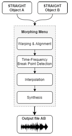
The original morphing algorithm was implemented as a five-stage procedure:

1. Extracting parameters (F0, aperiodicity and STRAIGHT spectrogram) of each utterance;
2. Warping and aligning time-frequency coordinates of parameters of two exemplar utterances;
3. Interpolating (and if necessary extrapolating) parameters represented on the aligned time-frequency coordinates according to the given morphing rate(s);
4. Deforming the time-frequency coordinates according to the given morphing rate(s); and
5. Re-synthesizing sound using the morphed parameters on the morphed time-frequency coordinate.

First, the extracted high-level features of two input audio files are warped to ensure that onsets and durations are properly aligned and then re-sampled at equal intervals to ensure that frames in both recordings correspond to one another.

Temporal interpolation involves alignment and rescaling. That means that after fixing the manually anchored points in the temporal domain, the dynamic time warping (DTW) algorithm is used to align the rest of the frames with each other. Usually, the lengths of the files are different (and so the spectrogram sizes), so the algorithm repeats the last frames in the spectrum to prevent any discontinuities or contractions from occurring in the resulting morphs.

Frequency interpolation involves matching and formants’ interpolation. Matching is a pre-interpolation stage used to form correspondences between harmonics in each sound sample. It involves looking for the harmonics closest in frequency (i.e., harmonic pairings) using a morphing matrix and seeking the best-matching harmonics frame-by-frame. Since formants are responsible for how speech sounds, it is crucial to identify and maintain that information. This is achieved by identifying each peak’s amplitude and frequency location. Based on that information and with the weighting function, the new intermediate formant location is derived. This process is repeated for any formants that fall within a specific frequency range. For the remainder of anchors, a simple one-to-one average cross-fade is sufficient. This step results in creating an intermediate spectral shape that can be applied to the amplitudes of all harmonics.

After the spectral and aperiodicity data have been analyzed, we can begin the final interpolation that utilizes all the information we computed. The corresponding features of two inputs and the new, interpolated values determine the amount of scaling required for the morphed features. There will be one morphed harmonic generated for every two contributing harmonics. Each morphed harmonic will contain the values of the contributing harmonics interpolated using the weighting function. The interpolated acoustic features will be reflected in the final, morphed output.

The final step is to re-synthesize all the interpolated high-level features to generate the morphed sound. This re-synthesis is based on a linear interpolation between the anchor templates of the two speech samples. This results in a single morphed sound file.

2.1. Initialising MorphingMenu module

To activate the morphing menu interface, type the following into the MATLAB Command Window: MorphingMenu. The following window should appear (see Figure 12). Only relevant buttons are accessible depending on the stage of processing

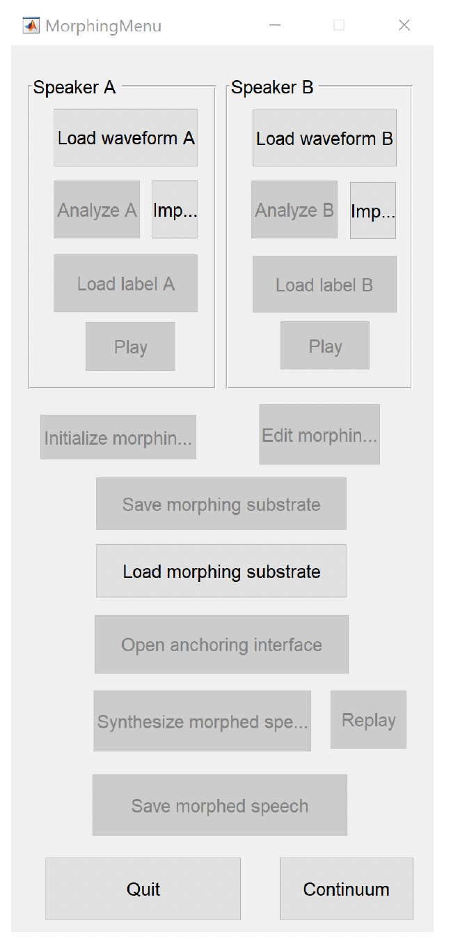
To begin the morphing procedure, you need to load the pre-analyzed .mat files (with the StrObj prefix/suffix) you generated in the previous step. To load the first file, press the Imp… (Select STRAIGHT object(A) to load) button under the Speaker A section. To load the second file, press the Imp… (Select STRAIGHT object(B) to load) button under the Speaker B section.

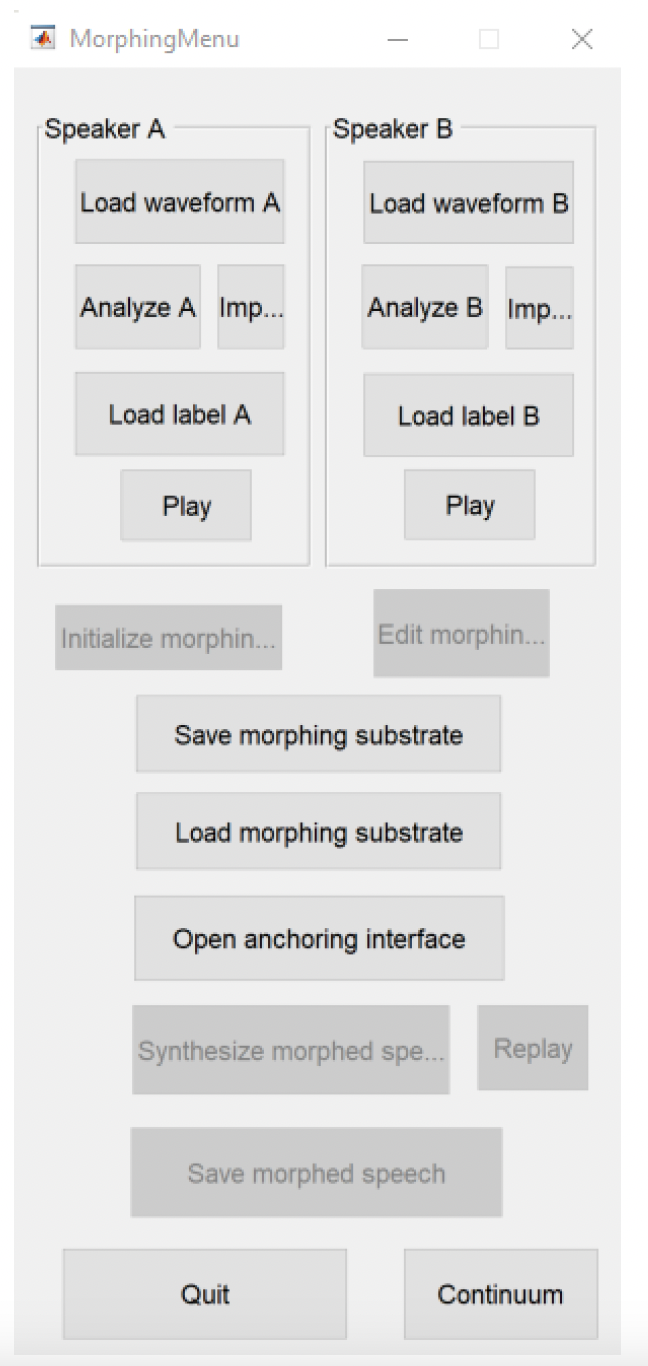
You can also load both wav files by pressing the Load waveform A and Load waveform B buttons and begin the analysis by clicking Analyze A or Analyze B, respectively. This will bring up the STRAIGHT analysis window. You cannot morph any speech samples without analyzing them first. After loading the .mat files, some additional options will become available (see Figure 13). For example, you can now listen to the uploaded files by pressing the Play button in the relevant section.

2.2. Aligning files with temporal anchor

Once the sounds are loaded, press the Open anchoring interface button to start the procedure of specifying the parameters that will be used for the alignment between the two speech samples. This might take a few seconds, so please be patient and don’t click any other buttons while MATLAB is processing your request. When ready, you will see a new window of the temporal anchor interface containing the two waveforms and spectrograms (with file A on the top and file B at the bottom) you just uploaded (see Figure 14). At this stage, you can click the Play A and Play B buttons to listen to your files.

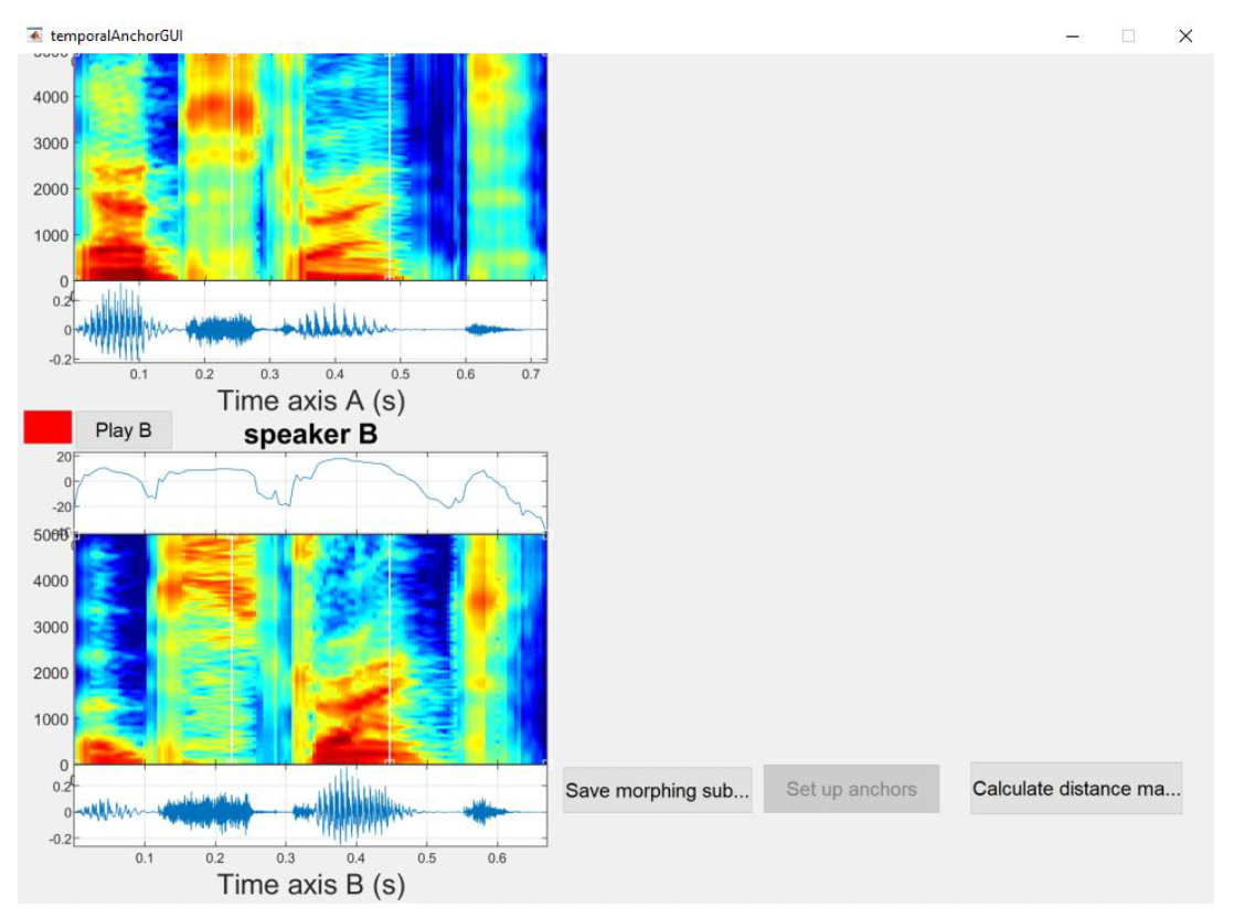
Note: The two plots on the left represent spectrograms of speech sample A and B with a power plot at the top and waveform on the bottom panel.

The first step is to click on the Calculate distance matrix button, which will compare each audio frame from one file to each frame in the other file. Again, this might take a few seconds, so please don't press any other buttons while MATLAB calculates the matrix. This generates the distance matrix, as shown in Figure 15.

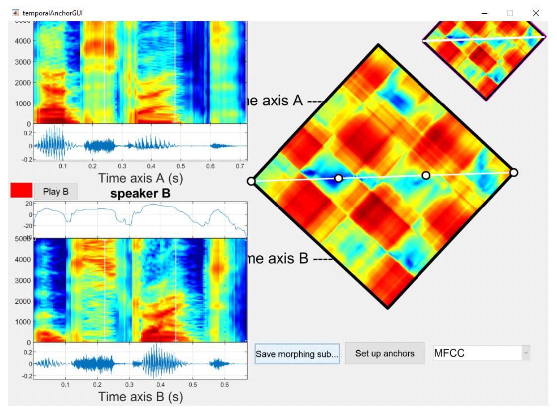
Note: The top right panel shows a smaller copy of the distance matrix to help with navigation. The bottom panel shows the zoomed distance matrix that is used to edit anchoring points. Both representations are rotated 45 degrees. Dark blue represents small distances (very similar frames of audio), and dark red represents large distances (very different frames of audio). By default, the distance matrix is calculated using MFCC features (Mel Frequency Cepstral Coefficients), but other options (Linear, Shift Invariant 1 and MFCCmod) can also be selected. MFCC distance is a recommended distance measurement for spectrum sequences. The shape of the vocal tract determines what sound comes out, so if we determine this shape accurately, we should obtain an accurate representation of speech being produced. The shape of the vocal tract manifests itself in the envelope of the short-time power spectrum, and MFCCs accurately represent that envelope. That is why MFCCs are widely used in speech recognition and are a good choice for calculating distance matrix for morphing.

In general, you will observe similar stripe or checkboard patterns, and the boundaries of these stripes correspond roughly to segment boundaries. The initial alignment is always a straight line across the two files. This should be pretty close to the path you’ll eventually choose because you want the resulting sound files to be as similar as possible to the files you are morphing together.

The temporal anchors should be placed such that they line up to points in the sound file that have the same meaning in both files. That means that the location and number of anchor points will depend on the speech sample itself.

We want to segment the utterances in some meaningful way with anchors placed at the beginning and end of each segment (i.e., onsets and offsets of vowels, consonants and silences) and supply at least a midpoint of each segment as an additional anchor (especially for longer pauses, extended vowels or diphthongs and consonant clusters). Since two speech samples may contain different segments, these have to be marked in both utterances to create congruent sequences of morphing anchors. The locations of these additional anchors must be selected carefully, optimally during pauses or adjacent sounds that have the same type of excitation (voiced or unvoiced) as the respective segment in the other utterance. Otherwise, noticeable artefacts can arise when the speech samples are mixed. In general, you want to mark clear changes in the spectra and midpoints of long vowels and sibilants.

To start setting up our temporal anchors, begin by looking at the distance matrix. The general path is usually pretty obvious, so you can place anchor points where you estimate the path to be. Start by marking where red rectangles in the upper and lower halves of the matrix meet at a corner. Then, use the zoom features to look closer across the path and again mark where the path seemed to be on a finer-grained level, where similarly coloured sections in the upper and lower halves meet at a corner.

Then, look at the anchor points with respect to where they appeared in the spectrograms of the individual wav files, and make sure they appeared at acoustically similar time points (i.e., the vertical white lines mark the onset, offset or midpoint of the selected speech events). To do that, play the input sounds and make sure that if you've marked (e.g.) the release of a /t/ in Sound A, that you are marking the same event in Sound B.

In cases where a segment is much longer in Sound A than Sound B, and this is a crucial contrast (e.g. stressed vs unstressed), make sure to use multiple anchor points for that section to try and be as accurate as possible. For example, you could place an anchor point at vowel onset, another halfway through the vowel, and another when the following consonant begins.

It is important to be careful where voicing begins and ends to make sure you're not morphing voiced and unvoiced time points.

You can adjust the temporal anchors in the magnified distance matrix on the right (white circles) or directly on the spectrograms of speech samples A and B (white lines). This step will require a lot of tweaking to align the two speech files well. See below for more details about how to interact with the temporal anchors’ interface.

Temporal anchoring interface controls:

• Zoom in/out
  • Click on the time axis of either sound file to zoom in
  • Hold shift and click on the time axis to zoom out
  • When zoomed in, you can click and drag the spectrograms, waveforms or distance matrix to move the visible areas
• Click on the white alignment line across the distance matrix to add a new anchor
  • Mouse cursor will change to have a plus
• Click and drag on an anchor to move it around (you can also click and drag the lines in the spectrogram view)
  • Hold shift and click to remove an anchor - mouse cursor will change to an eraser
  • Hold alt and click to bring up the frequency anchor interface - mouse cursor will change to a pointing hand

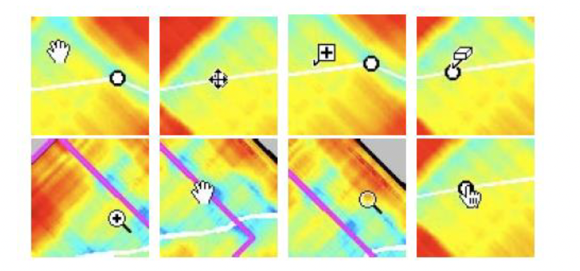
Note: The shapes of a pointer in matrix magnification mode represent their assigned functions. From top left to bottom right: distance matrix dragging (hand), anchor position modification (crossed arrows), addition of new anchor point (plus symbol), deletion of existing anchor point (eraser symbol), expansion of zoomed region (magnifier with a plus symbol), dragging inspection region (hand), relocation to the pointer position (empty magnifier) and inspection of spectral slices for frequency anchoring (pointing hand). These functions are dependent on graphic objects present under pointer and depression of modifier keys.

Once you are happy with your temporal anchors' alignment, you need to save them for further analysis. The assigned temporal anchor points are returned to the morphing menu by clicking the Set up anchors button.

2.3. Aligning files with frequency anchor (optional)

We can also set up frequency anchors for the sibilant and the formant transitions to make those sound more natural. Without frequency anchors, any differences will be mixed linearly in the frequency domain, similar to what you would get if you made the stimuli in Praat by extracting two sounds and mixing them at different percentages. Instead, we can shift the spectral peak around in STRAIGHT. The differences between mixing and shifting are not super pronounced when synthesizing sibilant continua but make a huge difference in synthesizing vowel continua (shifting formants around). Frequency anchoring points are set to minimize discrepancy of representative spectral features, such as formant frequencies.

As such, setting frequency anchors marking voiceless parts of the samples is not necessary. Placing frequency anchors at centre frequencies of formants (where detectable) at each time-anchor location of voiced part of speech are recommended (e.g., Skuk, Dammann & Schweinberger, 2015; Kachel et al., 2018). For better alignment, spectro-temporal anchors can be set at the onset of phonation, onset of formant transition, and end of phonation (Pernet & Belin, 2021). If more than one formant candidate falls within expected ranges, the one with the lowest bandwidth should be considered as the anchor frequency.

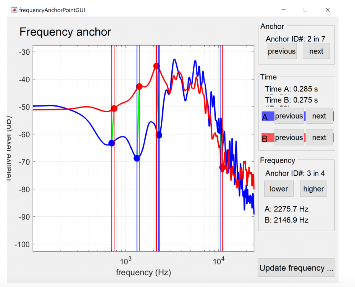
Once you have an anchor in the middle of the sound to be morphed, we want to anchor the peaks in the frequency domain. To do so, hold alt and click on the point in the centre of the voiced segment (the cursor will turn to a pointing hand over the anchor). This will bring up a display of the spectra for the two wave files at that point in time (see Figure 17).

Frequency anchoring interface controls:

• Zoom in/out
  • Click on the frequency axis of either sound file to zoom in
  • Hold shift and click to zoom out
  • Click and drag the white background to move the visible part of the spectrum
• Click on either frequency spectrum to add an anchor
  • Mouse cursor will change to have a plus
• Click and drag on the dots to change what parts of the spectrum are aligned
  • Hold shift and click to remove an anchor - mouse cursor will change to an eraser
  • Graphical elements can interfere with one another, so you may have to move something out of the way first

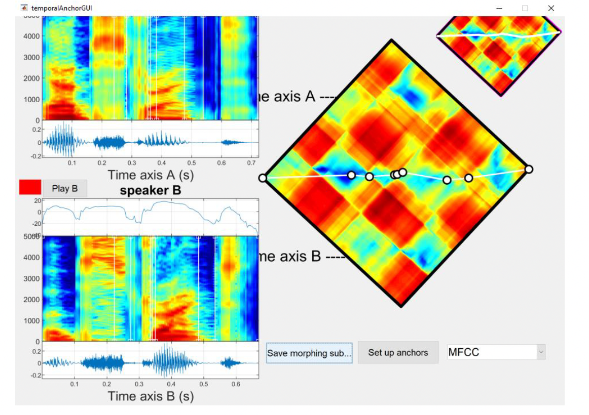
Once you’re happy with the frequency anchors, press the Update frequency anchors button in the lower right of the window, and that will save what you have anchored and pass it back to the main anchoring window. You will be redirected back to the TemporalAnchorGui below (see Figure 18). You will notice that updating the frequency anchors did not have any effect on the temporal anchors you set previously.

2.4. Setting up anchors

Once all the anchors are set up to your satisfaction, you can press the Set up anchors button to send the work back to the main morphing window. Pressing this button brings back the main MorphingMenu. To save your work, press the Save morphing substrate button and save the .mat file with a meaningful name so you can easily find it during the next steps of the analysis (e.g., word1and2_MorphSub.mat). You need to insert the suffix _MorphSub after your desired filename so that the MATLAB scripts can load this file when generating morphed audio. You can now close the TemporalAnchorGUI window.

At this stage, you can either continue your analyses by setting up morphing rates for new speech synthesis or save your work and return to it later. When you are ready to continue, you can open MorphingMenu by typing its name in the MATLAB command window and access the previously saved morphing substrate by pressing the Load morphing substrate button. Once loaded, you can continue with the analysis.

2.5. Setting up morphing rates

Once temporal and frequency anchoring is finished, or the morphing substrate mat file from a previous session is loaded, you’ll have to set up the two endpoints of the continuum you want to generate. This step will allow you to evaluate how well your files are aligned and check if the synthesized intermediate versions between the two speech samples sound natural.

There are two ways you might want to proceed with this:

1. You can explore the morphed version by manually setting the parameters across the selected acoustic dimensions to check the quality of the substrates and then use the previously saved morphing substrate defining the temporal and frequency anchor points between the two files in custom made scripts to automatically generate the stimuli along the defined continuum; or
2. Generate two morphing substrates, one for each end of the continuum and use these to synthesize the stimuli continuum with the makeMorphingContinuumGUI by defining the number of steps.

Either way, you need to explore how well your morphing works before proceeding further.

Note: Make sure to generate and listen to the output, and see what effect moving, adding, removing anchor points has on the synthesized speech. And be sure to generate "morphs" at the extremes you plan to use. (e.g., 90% pitch 10% duration) to make sure it still sounds natural.

For my research, I generate speech continua with MATLAB scripts (see Option 1 above). Nevertheless, I usually go through the whole procedure to generate the extremes of our continuum to check the quality of morphed speech before generating all samples. If the resulting speech samples do not sound natural, we’ll need to go back and adjust temporal and frequency anchors to make this work.

To start the morphing procedure, press the Initialize morphing rate button and then the Edit morphing rate button. This will open the morphing rate window (see Figure 19).

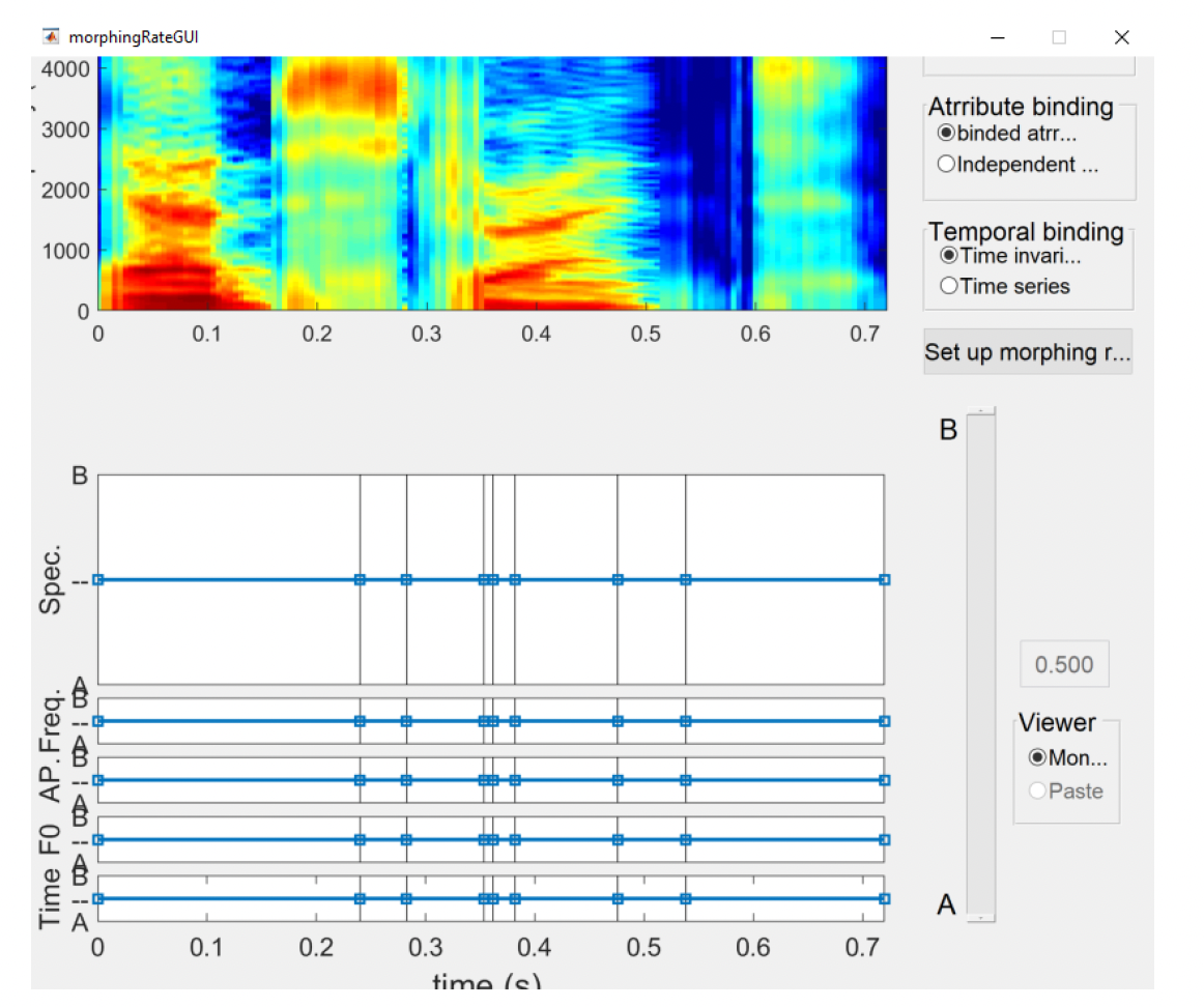
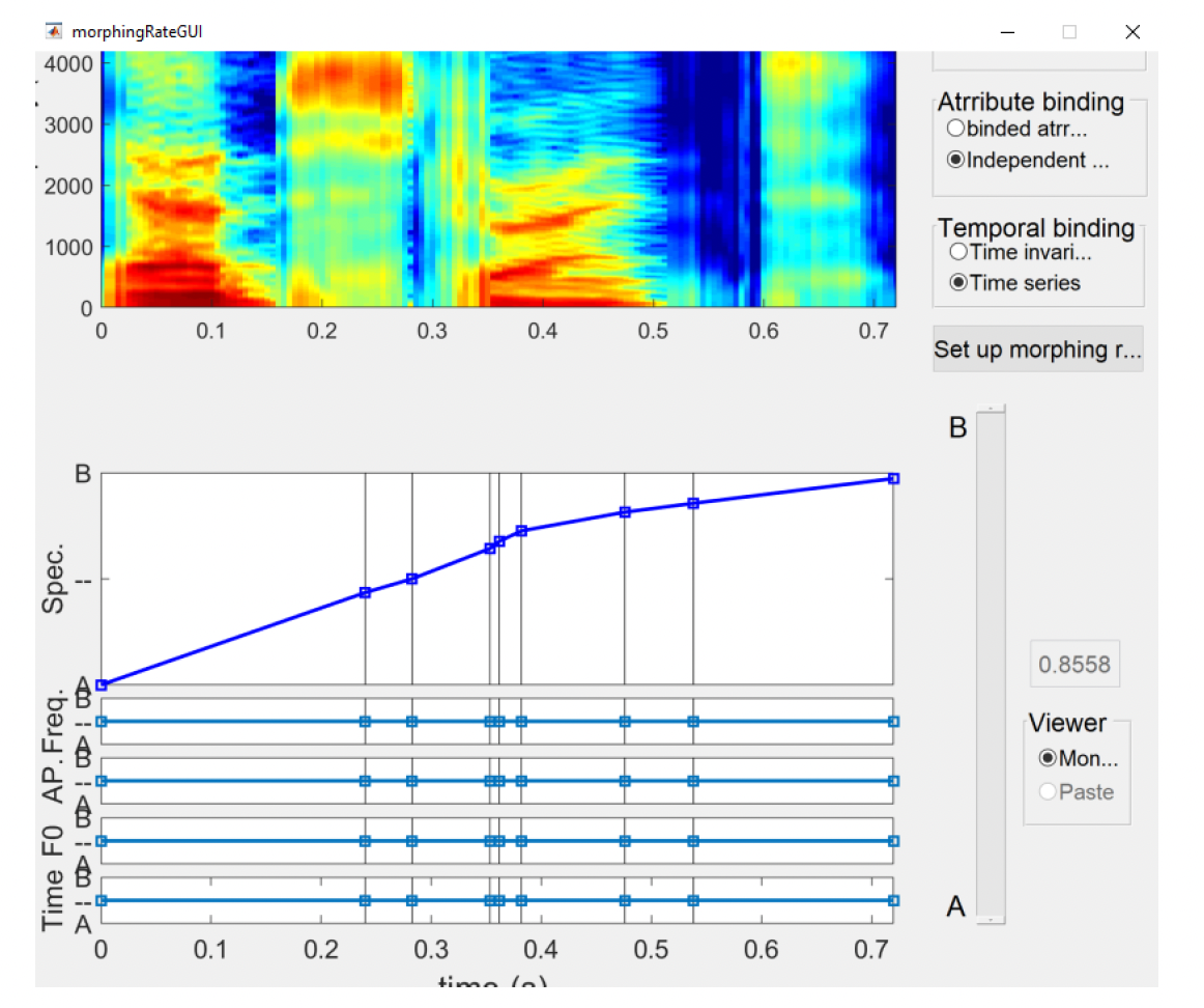
Note: This GUI consists of six plots; from top to bottom: STRAIGHT spectrogram, spectrum level morphing rate, frequency axis morphing rate, aperiodicity morphing rate, F0 morphing rate and temporal axis morphing rate. Similar to the STRAIGHT parameter manipulation GUI, the spectrographic display is used as a handle for zooming and dragging on the horizontal axis. The other five plots are used to assign morphing rates. The morphing procedure requires each of five aspects to be specified as a single or a multidimensional time series (Kawahara, Takahashi, Morise, & Banno, 2009).

The section titled Reference speaker allows you to choose whether morphing starts with reference to example A or B. When selecting the Time-invariant temporal binding, there is no difference in the output files (speech samples A and B are equally distributed over time in the output file). However, if we are using the Time series temporal binding parameter, this will define which file serves as a baseline sample (morphed from) and which one is a target sample (morphed to).

As mentioned above, the Temporal binding setting offers two options: (1) time-invariant and (2) time series. The time-invariant option maintains stable values of the selected features throughout the duration of the morphed speech sample (as expressed by straight vertical lines in Figure 18). Time series temporal binding allows you to implement gradual changes in each dimension over time, as shown in Figure 20.

For our purposes, we use the Time invariant temporal binding so that the values in each dimension remain stable throughout the generated speech sample.

The Attribute binding setting has two options: (1) binded attributes that modify the morphing rate of all features at the same time; and (2) independent attributes that modify the morphing rates independently for each selected dimension. Since we’ll be manipulating pitch and duration only, we want to select the Independent attributes option so that we can change the amount of information in each of these dimensions separately. The values of other morphing dimensions should be kept constant.

The vertical lines in those five plots represent temporal anchoring points. Morphing rates are represented by a piecewise linear function using temporal anchoring points as nodes of the function. Two types of anchoring point allocation are available: (1) drawing a line with a pen and (2) dragging a node group selected by region selection. In the case of line drawing, the crossing point at each temporal anchor is copied to the morphing rate value of the node point.

After selecting appropriate morphing rates across features, press the Set the morphing rate button to apply these settings (please wait for the button to become grey). To listen to the morphed speech sound, go back to the main MorphingMenu window and press the Synthesize morphed speech button. You can now hear your first morphed sample.

To generate morphing substrates for the extremes of the continuum, repeat the procedure with the appropriate settings defining both ends of the continuum and then click the Save morphing substrate button. Save two morphing substrates, one for each end of the continuum and name them in a meaningful way so you can easily find them (e.g., mSubstr-Word1.mat and mSubstr-Word2.mat). You can generate the corresponding wav files and check if the resulting files meet your expectations.

If you are happy with these, you are now ready to start generating the intermediate files of your continuum.

FAQ

What can I do with morphed stimuli?

The most common way to use STRAIGHT in speech perception experiments is to morph between two similar sound files that differ in a key way. In my experiments, I focused on differences in selected prosodic features - contrastive focus, phrase boundary and lexical stress.

References

Kawahara, H., Katayose, H., de Cheveigne, A., & Patterson, R. D. (1999). Fixed point analysis of frequency to instantaneous frequency mapping for accurate estimation of F0 and periodicity. Proceedings of the 6th European Conference on Speech Communication and Technology (EuroSpeech), 2781-2784.

Kawahara, H., Takahashi, T., Morise, M., & Banno, H. (2009). Development of exploratory research tools based on TANDEM-STRAIGHT. Proceedings of the Asia-Pacific Signal and Information Processing Association, Annual Summit and Conference (APSIPA ASC), 111-120.

Skuk, V. G., Dammann, L. M., & Schweinberger, S. R. (2015). Role of timbre and fundamental frequency in voice gender adaptation. The Journal of the Acoustical Society of America, 138, 1180-1193.

First published on: June 26, 2025